Time series
%matplotlib inline
Just checking the logic.
import matplotlib.pyplot as plt
from HJCFIT.likelihood import plot_time_series
from HJCFIT.likelihood.random import time_series as random_time_series

perfect, series = random_time_series(N=100, n=100, tau=1)
print(perfect)
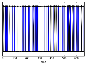
fig, ax = plt.subplots(1,1)
plot_time_series(perfect, ax=ax)
plot_time_series(series, ax=ax, marker='*', color='k', linestyle=':')
[   0.            8.59256356   13.17355631   22.65902932   30.51518269
   39.80841094   43.44484256   52.40072443   59.61475713   67.98731603
   76.4723764    80.89963682   90.84416819   96.54831984  105.41180332
  115.19328038  123.54596142  132.36917277  142.20242392  148.21030341
  158.20874751  161.38849311  170.48725632  176.4956325   185.39531444
  191.89856023  198.83685826  204.49651737  209.7973213   216.95273892
  221.05919062  229.65418582  238.26067727  241.70173579  245.65145402
  249.52013766  256.54599658  262.18962559  266.15962003  273.93633196
  283.39856545  286.70842402  296.25077954  305.3712874   313.01989332
  320.42691522  328.14012926  337.8075964   341.70598939  350.20743812
  353.38204688  362.27510626  371.70551543  375.2230498   384.61762256
  389.15553529  392.73575791  401.43023923  408.29600194  413.83360224
  417.92996481  423.7774031   432.98776285  442.64181207  449.18417602
  452.27298482  456.38927169  462.51919708  466.31855265  470.69058382
  480.14110632  484.75552799  490.97614438  493.98123983  502.03687601
  507.35256576  513.18612587  522.63779955  525.99850407  534.83319294
  539.53052581  546.00109775  551.15733842  557.08909557  562.36622206
  569.95964467  574.04627895  579.80772582  583.72298285  593.37151631
  600.4412491   607.52752039  612.33312193  616.38161548  624.81590068
  634.03294875  640.49775222  646.01028819  651.79184332  656.47139117
  663.41252658]
from HJCFIT.likelihood import time_filter as cpp_time_filter
filtered = cpp_time_filter(series, 1)
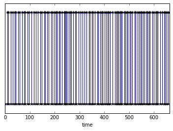
fig, ax = plt.subplots(1,1)
plot_time_series(perfect, ax=ax)
plot_time_series(filtered, ax=ax, marker='*', color='k', linestyle=':')
Now, computes the likelihood of this time series for a random QMatrix