CH82 Model¶

The following tries to reproduce Fig 8 from Hawkes, Jalali, Colquhoun (1992). First we create the \(Q\)-matrix for this particular model. Please note that the units are different from other publications.

%matplotlib inline

import numpy as np
import matplotlib.pyplot as plt

from dcprogs.likelihood import QMatrix

tau = 1e-4
qmatrix = QMatrix([[ -3050,        50,  3000,      0,    0 ],
                   [ 2./3., -1502./3.,     0,    500,    0 ],
                   [    15,         0, -2065,     50, 2000 ],
                   [     0,     15000,  4000, -19000,    0 ],
                   [     0,         0,    10,      0,  -10 ] ], 2)
qmatrix.matrix /= 1000.0

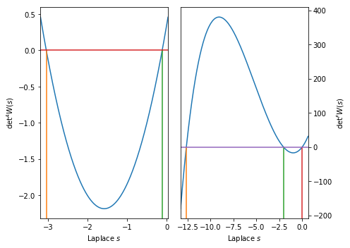
We first reproduce the top tow panels showing \(\mathrm{det} W(s)\) for open and shut times. These quantities can be accessed using dcprogs.likelihood.DeterminantEq. The plots are done using a standard plotting function from the dcprogs.likelihood package as well.

from dcprogs.likelihood import plot_roots, DeterminantEq

fig, ax = plt.subplots(1, 2, figsize=(7,5))

plot_roots(DeterminantEq(qmatrix, 0.2), ax=ax[0])
ax[0].set_xlabel('Laplace $s$')
ax[0].set_ylabel('$\\mathrm{det} ^{A}W(s)$')

plot_roots(DeterminantEq(qmatrix, 0.2).transpose(), ax=ax[1])
ax[1].set_xlabel('Laplace $s$')
ax[1].set_ylabel('$\\mathrm{det} ^{F}W(s)$')
ax[1].yaxis.tick_right()
ax[1].yaxis.set_label_position("right")

fig.tight_layout()

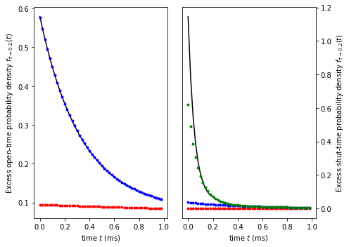
Then we want to plot the panels c and d showing the excess shut and open-time probability densities\((\tau = 0.2)\). To do this we need to access each exponential that makes up the approximate survivor function. We could use:

from dcprogs.likelihood import ApproxSurvivor
approx = ApproxSurvivor(qmatrix, tau)
components = approx.af_components
print(components[:1])

[(array([[  9.99994874e-01,  -1.96070450e-02],
       [ -2.61427266e-04,   5.12584244e-06]]), -3.050008571211625)]

The list components above contain 2-tuples with the weight (as a matrix) and the exponant (or root) for each exponential component in \(^{A}R_{\mathrm{approx}}(t)\). We could then create python functions pdf(t) for each exponential component, as is done below for the first root:

from dcprogs.likelihood import MissedEventsG

weight, root = components[1]
eG = MissedEventsG(qmatrix, tau)
# Note: the sum below is equivalent to a scalar product with u_F
coefficient = sum(np.dot(eG.initial_occupancies, np.dot(weight, eG.af_factor)))
pdf = lambda t: coefficient * exp((t)*root)

The initial occupancies, as well as the \(Q_{AF}e^{-Q_{FF}\tau}\) factor are obtained directly from the object implementing the weight, root = components[1] missed event likelihood \(^{e}G(t)\).

However, there is a convenience function that does all the above in the package. Since it is generally of little use, it is not currently exported to the dcprogs.likelihood namespace. So we create below a plotting function that uses it.

from dcprogs.likelihood._methods import exponential_pdfs

def plot_exponentials(qmatrix, tau, x=None, ax=None, nmax=2, shut=False):
    from dcprogs.likelihood import missed_events_pdf
    if ax is None:
        fig, ax = plt.subplots(1,1)
    if x is None: x = np.arange(0, 5*tau, tau/10)
    pdf = missed_events_pdf(qmatrix, tau, nmax=nmax, shut=shut)
    graphb = [x, pdf(x+tau), '-k']
    functions = exponential_pdfs(qmatrix, tau, shut=shut)
    plots = ['.r', '.b', '.g']
    together = None
    for f, p in zip(functions[::-1], plots):
        if together is None: together = f(x+tau)
        else: together = together + f(x+tau)
        graphb.extend([x, together, p])

    ax.plot(*graphb)

fig, ax = plt.subplots(1,2, figsize=(7,5))
ax[0].set_xlabel('time $t$ (ms)')
ax[0].set_ylabel('Excess open-time probability density $f_{\\bar{\\tau}=0.2}(t)$')
plot_exponentials(qmatrix, 0.2, shut=False, ax=ax[0])

plot_exponentials(qmatrix, 0.2, shut=True, ax=ax[1])
ax[1].set_xlabel('time $t$ (ms)')
ax[1].set_ylabel('Excess shut-time probability density $f_{\\bar{\\tau}=0.2}(t)$')
ax[1].yaxis.tick_right()
ax[1].yaxis.set_label_position("right")
fig.tight_layout()

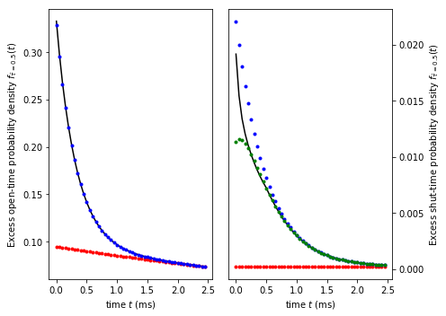
Finally, we create the last plot (e), and throw in an (f) for good measure.

fig, ax = plt.subplots(1,2, figsize=(7,5))
ax[0].set_xlabel('time $t$ (ms)')
ax[0].set_ylabel('Excess open-time probability density $f_{\\bar{\\tau}=0.5}(t)$')
plot_exponentials(qmatrix, 0.5, shut=False, ax=ax[0])

plot_exponentials(qmatrix, 0.5, shut=True, ax=ax[1])
ax[1].set_xlabel('time $t$ (ms)')
ax[1].set_ylabel('Excess shut-time probability density $f_{\\bar{\\tau}=0.5}(t)$')
ax[1].yaxis.tick_right()
ax[1].yaxis.set_label_position("right")

fig.tight_layout()

from dcprogs.likelihood import QMatrix, MissedEventsG

tau = 1e-4
qmatrix = QMatrix([[ -3050,        50,  3000,      0,    0 ],
                   [ 2./3., -1502./3.,     0,    500,    0 ],
                   [    15,         0, -2065,     50, 2000 ],
                   [     0,     15000,  4000, -19000,    0 ],
                   [     0,         0,    10,      0,  -10 ] ], 2)
eG = MissedEventsG(qmatrix, tau, 2, 1e-8, 1e-8)
meG = MissedEventsG(qmatrix, tau)
t = 3.5* tau

print(eG.initial_CHS_occupancies(t) -  meG.initial_CHS_occupancies(t))

[[  4.33877934e-12  -4.33864056e-12]]