HJCFIT- maximum likelihood fit of single-channel data:
Records at four concentrations fitted simultaneously
Some general settings:
%matplotlib inline
import matplotlib
import matplotlib.pyplot as plt
import sys, time, math
import numpy as np
from numpy import linalg as nplin
Load data
HJCFIT depends on DCPROGS/DCPYPS module for data input and setting kinetic mechanism:
from dcpyps.samples import samples
from dcpyps import dataset, mechanism, dcplots, dcio
# LOAD DATA: Burzomato 2004 example set.
scnfiles = [["./samples/glydemo/A-10.scn"],
            ["./samples/glydemo/B-30.scn"],
            ["./samples/glydemo/C-100.scn"],
            ["./samples/glydemo/D-1000.scn"]]
tr = [0.000030, 0.000030, 0.000030, 0.000030]
tc = [0.004, -1, -0.06, -0.02]
conc = [10e-6, 30e-6, 100e-6, 1000e-6]
Initialise Single-Channel Record from dcpyps. Note that SCRecord takes a list of file names; several SCN files from the same patch can be loaded.
# Initaialise SCRecord instance.
recs = []
bursts = []
for i in range(len(scnfiles)):
    rec = dataset.SCRecord(scnfiles[i], conc[i], tr[i], tc[i])
    recs.append(rec)
    bursts.append(rec.bursts.intervals())
    rec.printout()
 Data loaded from file: ./samples/glydemo/A-10.scn
Concentration of agonist = 10.000 microMolar
Resolution for HJC calculations = 30.0 microseconds
Critical gap length to define end of group (tcrit) = 4.000 milliseconds
    (defined so that all openings in a group prob come from same channel)
Initial and final vectors for bursts calculated asin Colquhoun, Hawkes & Srodzinski, (1996, eqs 5.8, 5.11).

Number of resolved intervals = 14553
Number of resolved periods = 12322

Number of open periods = 6161
Mean and SD of open periods = 1.288416455 +/- 1.982357659 ms
Range of open periods from 0.030309819 ms to 29.300385504 ms

Number of shut intervals = 6161
Mean and SD of shut periods = 69.358758628 +/- 259.539574385 ms
Range of shut periods from 0.030003177 ms to 6902.281761169 ms
Last shut period = 115.868724883 ms

Number of bursts = 1480
Average length = 6.106142638 ms
Range: 0.039 to 261.102 millisec
Average number of openings= 4.162837838


 Data loaded from file: ./samples/glydemo/B-30.scn
Concentration of agonist = 30.000 microMolar
Resolution for HJC calculations = 30.0 microseconds
Critical gap length to define end of group (tcrit) = -1000.000 milliseconds
    (defined so that all openings in a group prob come from same channel)
Initial and final vectors for are calculated as for steady state openings and shuttings (this involves a slight approximation at start and end of bursts that are defined by shut times that have been set as bad).

Number of resolved intervals = 15939
Number of resolved periods = 12580

Number of open periods = 6290
Mean and SD of open periods = 1.702516108 +/- 2.243856294 ms
Range of open periods from 0.030157962 ms to 24.172481848 ms

Number of shut intervals = 6290
Mean and SD of shut periods = 70.374920964 +/- 2950.499773026 ms
Range of shut periods from 0.030011479 ms to 194377.349853516 ms
Last shut period = 0.045992190 ms

Number of bursts = 6
Average length = 18819.672168031 ms
Range: 1522.551 to 43719.292 millisec
Average number of openings= 1048.333333333


 Data loaded from file: ./samples/glydemo/C-100.scn
Concentration of agonist = 100.000 microMolar
Resolution for HJC calculations = 30.0 microseconds
Critical gap length to define end of group (tcrit) = -60.000 milliseconds
    (defined so that all openings in a group prob come from same channel)
Initial and final vectors for are calculated as for steady state openings and shuttings (this involves a slight approximation at start and end of bursts that are defined by shut times that have been set as bad).

Number of resolved intervals = 15085
Number of resolved periods = 10306

Number of open periods = 5153
Mean and SD of open periods = 3.107396297 +/- 3.542747918 ms
Range of open periods from 0.030413088 ms to 46.681848165 ms

Number of shut intervals = 5153
Mean and SD of shut periods = 165.682286024 +/- 6593.143939972 ms
Range of shut periods from 0.030006107 ms to 386315.155029297 ms
Last shut period = 0.060205570 ms

Number of bursts = 12
Average length = 1513.309260650 ms
Range: 0.853 to 5742.387 millisec
Average number of openings= 429.416666667


 Data loaded from file: ./samples/glydemo/D-1000.scn
Concentration of agonist = 1000.000 microMolar
Resolution for HJC calculations = 30.0 microseconds
Critical gap length to define end of group (tcrit) = -20.000 milliseconds
    (defined so that all openings in a group prob come from same channel)
Initial and final vectors for are calculated as for steady state openings and shuttings (this involves a slight approximation at start and end of bursts that are defined by shut times that have been set as bad).

Number of resolved intervals = 11116
Number of resolved periods = 7948

Number of open periods = 3974
Mean and SD of open periods = 5.501930670 +/- 5.808946772 ms
Range of open periods from 0.031116215 ms to 54.734716301 ms

Number of shut intervals = 3974
Mean and SD of shut periods = 127.277284861 +/- 4903.965950012 ms
Range of shut periods from 0.030000978 ms to 293057.556152344 ms
Last shut period = 2.376423450 ms

Number of bursts = 19
Average length = 1176.491361390 ms
Range: 21.215 to 4484.782 millisec
Average number of openings= 209.157894737
Load demo mechanism (C&H82 numerical example)
# LOAD FLIP MECHANISM USED in Burzomato et al 2004
mecfn = "./samples/mec/demomec.mec"
version, meclist, max_mecnum = dcio.mec_get_list(mecfn)
mec = dcio.mec_load(mecfn, meclist[2][0])
# PREPARE RATE CONSTANTS.
# Fixed rates.
#fixed = np.array([False, False, False, False, False, False, False, True,
#    False, False, False, False, False, False])
for i in range(len(mec.Rates)):
    mec.Rates[i].fixed = False

# Constrained rates.
mec.Rates[21].is_constrained = True
mec.Rates[21].constrain_func = mechanism.constrain_rate_multiple
mec.Rates[21].constrain_args = [17, 3]
mec.Rates[19].is_constrained = True
mec.Rates[19].constrain_func = mechanism.constrain_rate_multiple
mec.Rates[19].constrain_args = [17, 2]
mec.Rates[16].is_constrained = True
mec.Rates[16].constrain_func = mechanism.constrain_rate_multiple
mec.Rates[16].constrain_args = [20, 3]
mec.Rates[18].is_constrained = True
mec.Rates[18].constrain_func = mechanism.constrain_rate_multiple
mec.Rates[18].constrain_args = [20, 2]
mec.Rates[8].is_constrained = True
mec.Rates[8].constrain_func = mechanism.constrain_rate_multiple
mec.Rates[8].constrain_args = [12, 1.5]
mec.Rates[13].is_constrained = True
mec.Rates[13].constrain_func = mechanism.constrain_rate_multiple
mec.Rates[13].constrain_args = [9, 2]
mec.update_constrains()
# Rates constrained by microscopic reversibility
mec.set_mr(True, 7, 0)
mec.set_mr(True, 14, 1)

# Update constrains
mec.update_constrains()
#Propose initial guesses different from recorded ones
initial_guesses = [5000.0, 500.0, 2700.0, 2000.0, 800.0, 15000.0, 300.0, 120000, 6000.0,
                   0.45E+09, 1500.0, 12000.0, 4000.0, 0.9E+09, 7500.0, 1200.0, 3000.0,
                   0.45E+07, 2000.0, 0.9E+07, 1000, 0.135E+08]

#initial_guesses = [3687.69, 6091.43, 2467.35, 32621.5, 7061.15, 129984., 1050.69, 20984., 3387.64,
#                   0.166224E+09, 20783.8, 6308.02, 2258.42, 0.332447E+09, 31335.4, 144.530, 831.686,
#                   0.620171E+06, 554.457, 0.124034E+07, 277.229, 0.186051E+07]

#initial_guesses = mec.unit_rates()
mec.set_rateconstants(initial_guesses)
mec.update_constrains()
mec.printout()
class dcpyps.Mechanism
Values of unit rates [1/sec]:
0   From AF*        to AF           alpha1          5000.0
1   From AF         to AF*          beta1           500.0
2   From A2F*       to A2F          alpha2          2700.0
3   From A2F        to A2F*         beta2           2000.0
4   From A3F*       to A3F          alpha3          800.0
5   From A3F        to A3F*         beta3           15000.0
6   From A3F        to A3R          gama3           300.0
7   From A3R        to A3F          delta3          120000.0
8   From A3F        to A2F          3kf(-3)         6000.0
9   From A2F        to A3F          kf(+3)          450000000.0
10  From A2F        to A2R          gama2           1500.0
11  From A2R        to A2F          delta2          12000.0
12  From A2F        to AF           2kf(-2)         4000.0
13  From AF         to A2F          2kf(+2)         900000000.0
14  From AF         to AR           gama1           7500.0
15  From AR         to AF           delta1          1200.0
16  From A3R        to A2R          3k(-3)          3000
17  From A2R        to A3R          k(+3)           4500000.0
18  From A2R        to AR           2k(-2)          2000
19  From AR         to A2R          2k(+2)          9000000.0
20  From AR         to R            k(-1)           1000
21  From R          to AR           3k(+1)          13500000.0

Conductance of state AF* (pS)  =      40

Conductance of state A2F* (pS)  =      40

Conductance of state A3F* (pS)  =      40

Number of open states = 3
Number of short-lived shut states (within burst) = 6
Number of long-lived shut states (between bursts) = 1
Number of desensitised states = 0

Number of cycles = 2
Cycle 0 is formed of states: A3R  A3F  A2F  A2R
    forward product = 4.860000000e+18
    backward product = 4.860000000e+18
Cycle 1 is formed of states: AF  A2F  A2R  AR
    forward product = 3.240000000e+18
    backward product = 3.240000000e+18
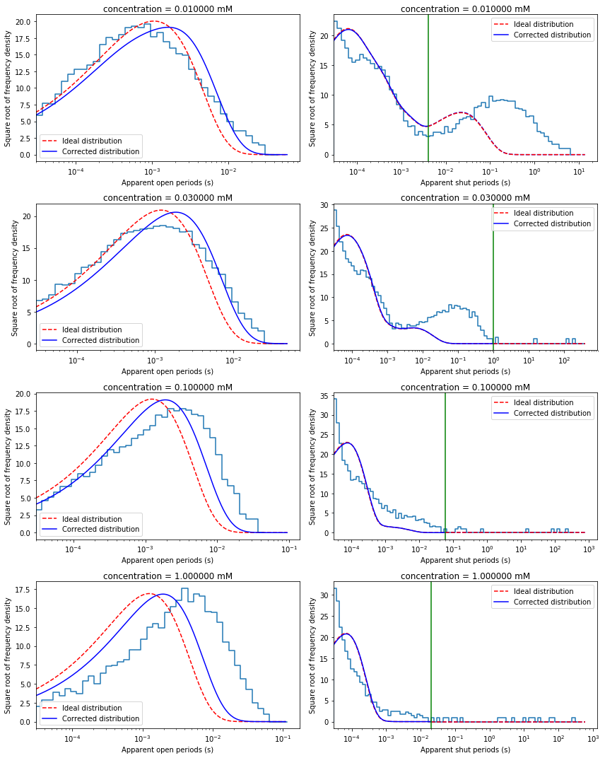
Check data histograms and probability densities calculated from initial guesses
Plot dwell-time histograms for inspection. In single-channel analysis field it is common to plot these histograms with x-axis in log scale and y-axis in square-root scale. After such transformation exponential pdf has a bell-shaped form.
Note that to properly overlay ideal and missed-event corrected pdfs ideal pdf has to be scaled (need to renormailse to 1 the area under pdf from \(\tau_{res}\)).
# Scale for ideal pdf
def scalefac(tres, matrix, phiA):
    eigs, M = eig(-matrix)
    N = inv(M)
    k = N.shape[0]
    A, w = np.zeros((k, k, k)), np.zeros(k)
    for i in range(k):
        A[i] = np.dot(M[:, i].reshape(k, 1), N[i].reshape(1, k))
    for i in range(k):
        w[i] = np.dot(np.dot(np.dot(phiA, A[i]), (-matrix)), np.ones((k, 1)))
    return 1 / np.sum((w / eigs) * np.exp(-tres * eigs))
from dcprogs.likelihood import QMatrix
from dcprogs.likelihood import missed_events_pdf, ideal_pdf, IdealG, eig, inv
fig, axes = plt.subplots(len(recs), 2, figsize=(12,15))
for i in range(len(recs)):
    mec.set_eff('c', recs[i].conc)
    qmatrix = QMatrix(mec.Q, mec.kA)
    idealG = IdealG(qmatrix)

    # Plot apparent open period histogram
    ipdf = ideal_pdf(qmatrix, shut=False)
    iscale = scalefac(recs[i].tres, qmatrix.aa, idealG.initial_occupancies)
    epdf = missed_events_pdf(qmatrix, recs[i].tres, nmax=2, shut=False)
    dcplots.xlog_hist_HJC_fit(axes[i,0], recs[i].tres, recs[i].opint,
                               epdf, ipdf, iscale, shut=False)
    axes[i,0].set_title('concentration = {0:3f} mM'.format(recs[i].conc*1000))

    # Plot apparent shut period histogram
    ipdf = ideal_pdf(qmatrix, shut=True)
    iscale = scalefac(recs[i].tres, qmatrix.ff, idealG.final_occupancies)
    epdf = missed_events_pdf(qmatrix, recs[i].tres, nmax=2, shut=True)
    dcplots.xlog_hist_HJC_fit(axes[i,1], recs[i].tres, recs[i].shint,
                               epdf, ipdf, iscale, tcrit=math.fabs(recs[i].tcrit))
    axes[i,1].set_title('concentration = {0:6f} mM'.format(recs[i].conc*1000))

fig.tight_layout()
Prepare likelihood function
def dcprogslik(x, lik, m, c):
    m.theta_unsqueeze(np.exp(x))
    l = 0
    for i in range(len(c)):
        m.set_eff('c', c[i])
        l += lik[i](m.Q)
    return -l * math.log(10)
def printiter(theta):
    global iternum, likelihood, mec, conc
    iternum += 1
    if iternum % 100 == 0:
        lik = dcprogslik(theta, likelihood, mec, conc)
        print("iteration # {0:d}; log-lik = {1:.6f}".format(iternum, -lik))
        print(np.exp(theta))
# Import HJCFIT likelihood function
from dcprogs.likelihood import Log10Likelihood

kwargs = {'nmax': 2, 'xtol': 1e-12, 'rtol': 1e-12, 'itermax': 100,
    'lower_bound': -1e6, 'upper_bound': 0}
likelihood = []

for i in range(len(recs)):
    likelihood.append(Log10Likelihood(bursts[i], mec.kA,
        recs[i].tres, recs[i].tcrit, **kwargs))
# Extract free parameters
theta = mec.theta()
print ('\ntheta=', theta)
print('Number of free parameters = ', len(theta))
theta= [  5.00000000e+03   5.00000000e+02   2.70000000e+03   2.00000000e+03
   8.00000000e+02   1.50000000e+04   3.00000000e+02   4.50000000e+08
   1.50000000e+03   1.20000000e+04   4.00000000e+03   1.20000000e+03
   4.50000000e+06   1.00000000e+03]
Number of free parameters =  14
lik = dcprogslik(np.log(theta), likelihood, mec, conc)
print ("\nInitial likelihood = {0:.6f}".format(-lik))
Initial likelihood = 237961.490136
Run optimisation
To keep execution time of this notebook short we only run the
optimization for 200 iterations. Change maxiter below for a more
realistic optimisation.
from scipy.optimize import minimize
print ("\nScyPy.minimize (Nelder-Mead) Fitting started: " +
       "%4d/%02d/%02d %02d:%02d:%02d"%time.localtime()[0:6])
iternum = 0
start = time.clock()
start_wall = time.time()
maxiter = 200
# maxiter = 30000
result = minimize(dcprogslik, np.log(theta), args=(likelihood, mec, conc), method='Nelder-Mead', callback=printiter,
                  options={'xtol':1e-5, 'ftol':1e-5, 'maxiter': maxiter, 'maxfev': 150000, 'disp': True})
t3 = time.clock() - start
t3_wall = time.time() - start_wall
print ("\nScyPy.minimize (Nelder-Mead) Fitting finished: " +
       "%4d/%02d/%02d %02d:%02d:%02d"%time.localtime()[0:6])
print ('\nCPU time in ScyPy.minimize (Nelder-Mead)=', t3)
print ('Wall clock time in ScyPy.minimize (Nelder-Mead)=', t3_wall)
print ('\nResult   ==========================================\n', result)
ScyPy.minimize (Nelder-Mead) Fitting started: 2016/10/28 15:27:05
iteration # 100; log-lik = 263117.756238
[  5.29171999e+03   3.67684624e+02   1.41434237e+03   8.42349605e+03
   8.62838471e+02   5.14562348e+04   3.05197111e+02   5.19871117e+07
   2.31972504e+03   2.00532661e+04   4.15472395e+03   5.07080801e+02
   5.01742534e+05   8.94263677e+02]
Warning: Maximum number of iterations has been exceeded.

ScyPy.minimize (Nelder-Mead) Fitting finished: 2016/10/28 15:27:15

CPU time in ScyPy.minimize (Nelder-Mead)= 19.19824
Wall clock time in ScyPy.minimize (Nelder-Mead)= 9.663951873779297

Result   ==========================================
  final_simplex: (array([[  8.17854356,   6.03708337,   7.10706279,   9.07985218,
          6.93061081,  10.98001309,   5.8136173 ,  17.23832524,
          7.72769902,   9.70103791,   8.19758666,   6.45112468,
         13.39684638,   6.95508465],
       [  8.22403089,   6.05593405,   7.12875747,   9.02313412,
          6.90356027,  10.95712368,   5.77448477,  17.24438837,
          7.73601058,   9.73603764,   8.23203859,   6.49199196,
         13.35532125,   6.97085489],
       [  8.27202446,   6.03124292,   7.15576058,   9.10298967,
          6.91537324,  10.97906583,   5.87535892,  17.27877025,
          7.7104076 ,   9.78828276,   8.22704485,   6.37777004,
         13.25294199,   6.93122741],
       [  8.32433001,   6.0289382 ,   7.1404883 ,   9.0383547 ,
          6.8205307 ,  10.93158792,   5.8308612 ,  17.34019634,
          7.75095584,   9.72800377,   8.25944946,   6.38964771,
         13.31653367,   6.93631765],
       [  8.33985033,   5.92301082,   7.09702954,   9.09805489,
          6.89673942,  10.97621154,   5.77517881,  17.32273873,
          7.74756632,   9.81249292,   8.25085744,   6.39354715,
         13.28852029,   6.94056203],
       [  8.41575544,   5.94125291,   7.19042536,   9.0435014 ,
          6.84337862,  10.89976979,   5.76975737,  17.40977212,
          7.775724  ,   9.77032599,   8.30672733,   6.40129054,
         13.28746099,   6.87193334],
       [  8.23460356,   6.06544835,   7.15047868,   9.05344456,
          6.87980573,  10.9657658 ,   5.76339175,  17.33221254,
          7.74893403,   9.78425826,   8.27631384,   6.45009588,
         13.17781919,   6.88956063],
       [  8.39823157,   5.92139609,   7.126189  ,   9.0460798 ,
          6.85351439,  10.9340107 ,   5.72892779,  17.42246383,
          7.78649285,   9.77082672,   8.31723055,   6.38863181,
         13.28356059,   6.92208135],
       [  8.41035142,   6.01081853,   7.19216558,   8.99209568,
          6.81683175,  10.90190722,   5.76531268,  17.4582171 ,
          7.77716363,   9.72993475,   8.33889227,   6.42272102,
         13.29925003,   6.88808181],
       [  8.40340552,   6.0273153 ,   7.22178376,   9.03888376,
          6.84264901,  10.91086406,   5.79190033,  17.45077881,
          7.73933892,   9.80968022,   8.24822381,   6.33622711,
         13.28545754,   6.9169019 ],
       [  8.24388707,   6.05157538,   7.20532864,   8.941294  ,
          6.84121632,  10.89460159,   5.76758747,  17.41789114,
          7.74027848,   9.70505269,   8.28434299,   6.52015363,
         13.39744932,   6.94780185],
       [  8.27610963,   6.05970142,   7.18039864,   9.13973644,
          6.87300261,  10.92971067,   5.93330882,  17.26117058,
          7.73212301,   9.73937094,   8.24832269,   6.4324554 ,
         13.1763455 ,   6.87493238],
       [  8.38279112,   5.8842607 ,   7.13565288,   9.0174619 ,
          6.84330267,  10.88373368,   5.78974106,  17.45101242,
          7.79970867,   9.74499968,   8.29915767,   6.43571606,
         13.37719486,   6.93389061],
       [  8.42420488,   5.88127595,   7.11098537,   9.09632685,
          6.83661948,  10.95519365,   5.74824873,  17.27662587,
          7.8087689 ,   9.797293  ,   8.31344718,   6.37128333,
         13.36240644,   6.92608137],
       [  8.4266003 ,   5.96016415,   7.18559361,   9.00606597,
          6.85428849,  10.93451427,   5.8372125 ,  17.29392659,
          7.78143967,   9.70305234,   8.3055485 ,   6.46089968,
         13.39443632,   6.98429024]]), array([-263352.60977117, -263336.3471002 , -263329.21681918,
       -263318.1251304 , -263309.78955037, -263306.30534451,
       -263302.2583715 , -263298.52765242, -263298.30026063,
       -263297.42510587, -263292.18626348, -263291.93074637,
       -263291.13476093, -263287.65737164, -263287.20390461]))
           fun: -263352.60977116873
       message: 'Maximum number of iterations has been exceeded.'
          nfev: 281
           nit: 200
        status: 2
       success: False
             x: array([  8.17854356,   6.03708337,   7.10706279,   9.07985218,
         6.93061081,  10.98001309,   5.8136173 ,  17.23832524,
         7.72769902,   9.70103791,   8.19758666,   6.45112468,
        13.39684638,   6.95508465])
print ("\nFinal likelihood = {0:.16f}".format(-result.fun))
mec.theta_unsqueeze(np.exp(result.x))
print ("\nFinal rate constants:")
mec.printout()
Final likelihood = 263352.6097711687325500

Final rate constants:

class dcpyps.Mechanism
Values of unit rates [1/sec]:
0   From AF*        to AF           alpha1          3563.66062627
1   From AF         to AF*          beta1           418.670145871
2   From A2F*       to A2F          alpha2          1220.55723999
3   From A2F        to A2F*         beta2           8776.66858648
4   From A3F*       to A3F          alpha3          1023.11872432
5   From A3F        to A3F*         beta3           58689.3222512
6   From A3F        to A3R          gama3           334.828110598
7   From A3R        to A3F          delta3          64801.2535522
8   From A3F        to A2F          3kf(-3)         5448.26105245
9   From A2F        to A3F          kf(+3)          30655579.3113
10  From A2F        to A2R          gama2           2270.3721034
11  From A2R        to A2F          delta2          16334.5522045
12  From A2F        to AF           2kf(-2)         3632.17403497
13  From AF         to A2F          2kf(+2)         61311158.6227
14  From AF         to AR           gama1           2368.25771823
15  From AR         to AF           delta1          633.414278499
16  From A3R        to A2R          3k(-3)          3145.40186848
17  From A2R        to A3R          k(+3)           657925.10102
18  From A2R        to AR           2k(-2)          2096.93457899
19  From AR         to A2R          2k(+2)          1315850.20204
20  From AR         to R            k(-1)           1048.46728949
21  From R          to AR           3k(+1)          1973775.30306

Conductance of state AF* (pS)  =      40

Conductance of state A2F* (pS)  =      40

Conductance of state A3F* (pS)  =      40

Number of open states = 3
Number of short-lived shut states (within burst) = 6
Number of long-lived shut states (between bursts) = 1
Number of desensitised states = 0

Number of cycles = 2
Cycle 0 is formed of states: A3R  A3F  A2F  A2R
    forward product = 5.273692624e+17
    backward product = 5.273692624e+17
Cycle 1 is formed of states: AF  A2F  A2R  AR
    forward product = 1.848882431e+17
    backward product = 1.848882431e+17
Plot experimental histograms and predicted pdfs
fig, axes = plt.subplots(len(recs), 2, figsize=(12,15))
for i in range(len(recs)):
    mec.set_eff('c', recs[i].conc)
    qmatrix = QMatrix(mec.Q, mec.kA)
    idealG = IdealG(qmatrix)

    # Plot apparent open period histogram
    ipdf = ideal_pdf(qmatrix, shut=False)
    iscale = scalefac(recs[i].tres, qmatrix.aa, idealG.initial_occupancies)
    epdf = missed_events_pdf(qmatrix, recs[i].tres, nmax=2, shut=False)
    dcplots.xlog_hist_HJC_fit(axes[i,0], recs[i].tres, recs[i].opint,
                               epdf, ipdf, iscale, shut=False)
    axes[i,0].set_title('concentration = {0:3f} mM'.format(conc[i]*1000))

    # Plot apparent shut period histogram
    ipdf = ideal_pdf(qmatrix, shut=True)
    iscale = scalefac(recs[i].tres, qmatrix.ff, idealG.final_occupancies)
    epdf = missed_events_pdf(qmatrix, recs[i].tres, nmax=2, shut=True)
    dcplots.xlog_hist_HJC_fit(axes[i,1], recs[i].tres, recs[i].shint,
                               epdf, ipdf, iscale, tcrit=math.fabs(recs[i].tcrit))
    axes[i,1].set_title('concentration = {0:6f} mM'.format(conc[i]*1000))

fig.tight_layout()
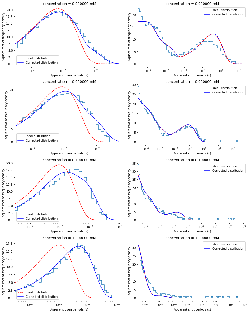
Note that in this record only shut time intervals shorter than critical time (\(t_{crit}\)) were used to minimise likelihood. Thus, only a part of shut time histrogram (to the left from green line, indicating \(t_{crit}\) value, in the above plot) is predicted well by rate constant estimates.