HJCFIT- maximum likelihood fit of single-channel data: a simple example
Some general settings:
%matplotlib inline
import matplotlib.pyplot as plt
import sys, time, math
import numpy as np
from dcprogs.likelihood import inv
Load data
HJCFIT depends on DCPROGS/DCPYPS module for data input and setting kinetic mechanism:
from dcpyps.samples import samples
from dcpyps import dataset, mechanism, dcplots
fname = "CH82.scn" # binary SCN file containing simulated idealised single-channel open/shut intervals
tr = 1e-4 # temporal resolution to be imposed to the record
tc = 4e-3 # critical time interval to cut the record into bursts
conc = 100e-9 # agonist concentration
Initialise Single-Channel Record from dcpyps. Note that SCRecord takes a list of file names; several SCN files from the same patch can be loaded.
# Initaialise SCRecord instance.
rec = dataset.SCRecord([fname], conc, tres=tr, tcrit=tc)
rec.printout()
 Data loaded from file: CH82.scn
Concentration of agonist = 0.100 microMolar
Resolution for HJC calculations = 100.0 microseconds
Critical gap length to define end of group (tcrit) = 4.000 milliseconds
    (defined so that all openings in a group prob come from same channel)
Initial and final vectors for bursts calculated asin Colquhoun, Hawkes & Srodzinski, (1996, eqs 5.8, 5.11).

Number of resolved intervals = 1672
Number of resolved periods = 1672

Number of open periods = 836
Mean and SD of open periods = 5.703315580 +/- 6.217026586 ms
Range of open periods from 0.101663936 ms to 36.745440215 ms

Number of shut intervals = 836
Mean and SD of shut periods = 2843.529462814 +/- 3982.407808304 ms
Range of shut periods from 0.100163714 ms to 30754.167556763 ms
Last shut period = 3821.345090866 ms

Number of bursts = 572
Average length = 8.425049759 ms
Range: 0.102 to 62.906 millisec
Average number of openings= 1.461538462
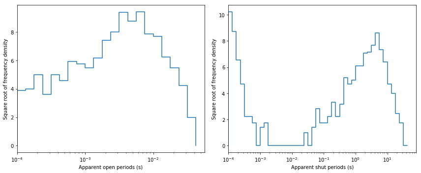
Plot dwell-time histograms for inspection. In single-channel analysis field it is common to plot these histograms with x-axis in log scale and y-axis in square-root scale. After such transformation exponential pdf has a bell-shaped form.
fig, ax  = plt.subplots(1, 2, figsize=(12,5))

dcplots.xlog_hist_data(ax[0], rec.opint, rec.tres, shut=False)

dcplots.xlog_hist_data(ax[1], rec.shint, rec.tres)

fig.tight_layout()
Load demo mechanism (C&H82 numerical example)
mec = samples.CH82()
mec.printout()
class dcpyps.Mechanism
Values of unit rates [1/sec]:
0   From AR         to AR*          beta1           15.0
1   From A2R        to A2R*         beta2           15000.0
2   From AR*        to AR           alpha1          3000.0
3   From A2R*       to A2R          alpha2          500.0
4   From AR         to R            k(-1)           2000.0
5   From A2R        to AR           2k(-2)          4000.0
6   From R          to AR           2k(+1)          100000000.0
7   From AR*        to A2R*         k*(+2)          500000000.0
8   From AR         to A2R          k(+2)           500000000.0
9   From A2R*       to AR*          2k*(-2)         0.66667

Conductance of state AR* (pS)  =      60

Conductance of state A2R* (pS)  =      60

Number of open states = 2
Number of short-lived shut states (within burst) = 2
Number of long-lived shut states (between bursts) = 1
Number of desensitised states = 0

Number of cycles = 1
Cycle 0 is formed of states: A2R*  AR*  AR  A2R
    forward product = 1.500007500e+16
    backward product = 1.500000000e+16
# PREPARE RATE CONSTANTS.
# Fixed rates
mec.Rates[7].fixed = True
# Constrained rates
mec.Rates[5].is_constrained = True
mec.Rates[5].constrain_func = mechanism.constrain_rate_multiple
mec.Rates[5].constrain_args = [4, 2]
mec.Rates[6].is_constrained = True
mec.Rates[6].constrain_func = mechanism.constrain_rate_multiple
mec.Rates[6].constrain_args = [8, 2]
# Rates constrained by microscopic reversibility
mec.set_mr(True, 9, 0)
# Update rates
mec.update_constrains()
#Propose initial guesses different from recorded ones
#initial_guesses = [100, 3000, 10000, 100, 1000, 1000, 1e+7, 5e+7, 6e+7, 10]
initial_guesses = mec.unit_rates()
mec.set_rateconstants(initial_guesses)
mec.update_constrains()
mec.printout()
class dcpyps.Mechanism
Values of unit rates [1/sec]:
0   From AR         to AR*          beta1           15.0
1   From A2R        to A2R*         beta2           15000.0
2   From AR*        to AR           alpha1          3000.0
3   From A2R*       to A2R          alpha2          500.0
4   From AR         to R            k(-1)           2000.0
5   From A2R        to AR           2k(-2)          4000.0
6   From R          to AR           2k(+1)          1000000000.0
7   From AR*        to A2R*         k*(+2)          500000000.0
8   From AR         to A2R          k(+2)           500000000.0
9   From A2R*       to AR*          2k*(-2)         0.666666666667

Conductance of state AR* (pS)  =      60

Conductance of state A2R* (pS)  =      60

Number of open states = 2
Number of short-lived shut states (within burst) = 2
Number of long-lived shut states (between bursts) = 1
Number of desensitised states = 0

Number of cycles = 1
Cycle 0 is formed of states: A2R*  AR*  AR  A2R
    forward product = 1.500000000e+16
    backward product = 1.500000000e+16
# Extract free parameters
theta = mec.theta()
print ('\ntheta=', theta)
theta= [  1.50000000e+01   1.50000000e+04   3.00000000e+03   5.00000000e+02
   2.00000000e+03   5.00000000e+08]
Prepare likelihood function
def dcprogslik(x, lik, m, c):
    m.theta_unsqueeze(np.exp(x))
    l = 0
    for i in range(len(c)):
        m.set_eff('c', c[i])
        l += lik[i](m.Q)
    return -l * math.log(10)
# Import HJCFIT likelihood function
from dcprogs.likelihood import Log10Likelihood

# Get bursts from the record
bursts = rec.bursts.intervals()
# Initiate likelihood function with bursts, number of open states,
# temporal resolution and critical time interval
likelihood = Log10Likelihood(bursts, mec.kA, tr, tc)
lik = dcprogslik(np.log(theta), [likelihood], mec, [conc])
print ("\nInitial likelihood = {0:.6f}".format(-lik))
Initial likelihood = 5264.414344
Run optimisation
from scipy.optimize import minimize
print ("\nScyPy.minimize (Nelder-Mead) Fitting started: " +
       "%4d/%02d/%02d %02d:%02d:%02d"%time.localtime()[0:6])
start = time.clock()
start_wall = time.time()
result = minimize(dcprogslik, np.log(theta), args=([likelihood], mec, [conc]),
               method='Nelder-Mead')
t3 = time.clock() - start
t3_wall = time.time() - start_wall
print ("\nScyPy.minimize (Nelder-Mead) Fitting finished: " +
       "%4d/%02d/%02d %02d:%02d:%02d"%time.localtime()[0:6])
print ('\nCPU time in ScyPy.minimize (Nelder-Mead)=', t3)
print ('Wall clock time in ScyPy.minimize (Nelder-Mead)=', t3_wall)
print ('\nResult   ==========================================\n', result)
ScyPy.minimize (Nelder-Mead) Fitting started: 2016/10/28 15:26:49

ScyPy.minimize (Nelder-Mead) Fitting finished: 2016/10/28 15:26:50

CPU time in ScyPy.minimize (Nelder-Mead)= 1.1934069999999997
Wall clock time in ScyPy.minimize (Nelder-Mead)= 0.5975382328033447

Result   ==========================================
  final_simplex: (array([[  2.33189798,   9.48999371,   8.20461943,   6.05142787,
          7.68244318,  19.98586637],
       [  2.33189349,   9.4899828 ,   8.20463764,   6.05141417,
          7.68244086,  19.98586557],
       [  2.33189951,   9.48998465,   8.20463814,   6.05141301,
          7.68245471,  19.98587732],
       [  2.33197072,   9.48998516,   8.20466661,   6.05141671,
          7.68245672,  19.98595769],
       [  2.33192346,   9.48994174,   8.20463429,   6.05137283,
          7.68245989,  19.98590225],
       [  2.33185111,   9.48999371,   8.20457848,   6.05142289,
          7.68244199,  19.98585741],
       [  2.33199047,   9.48997486,   8.20460338,   6.05139678,
          7.68245295,  19.98593748]]), array([-5268.59140924, -5268.59140923, -5268.59140923, -5268.59140921,
       -5268.5914092 , -5268.59140918, -5268.59140918]))
           fun: -5268.5914092352723
       message: 'Optimization terminated successfully.'
          nfev: 415
           nit: 256
        status: 0
       success: True
             x: array([  2.33189798,   9.48999371,   8.20461943,   6.05142787,
         7.68244318,  19.98586637])
print ("\nFinal likelihood = {0:.16f}".format(-result.fun))
mec.theta_unsqueeze(np.exp(result.x))
print ("\nFinal rate constants:")
mec.printout()
Final likelihood = 5268.5914092352722946

Final rate constants:

class dcpyps.Mechanism
Values of unit rates [1/sec]:
0   From AR         to AR*          beta1           10.2974673884
1   From A2R        to A2R*         beta2           13226.7121605
2   From AR*        to AR           alpha1          3657.80834791
3   From A2R*       to A2R          alpha2          424.719039018
4   From AR         to R            k(-1)           2169.9147908
5   From A2R        to AR           2k(-2)          4339.82958159
6   From R          to AR           2k(+1)          956712565.145
7   From AR*        to A2R*         k*(+2)          500000000.0
8   From AR         to A2R          k(+2)           478356282.573
9   From A2R*       to AR*          2k*(-2)         0.410062923425

Conductance of state AR* (pS)  =      60

Conductance of state A2R* (pS)  =      60

Number of open states = 2
Number of short-lived shut states (within burst) = 2
Number of long-lived shut states (between bursts) = 1
Number of desensitised states = 0

Number of cycles = 1
Cycle 0 is formed of states: A2R*  AR*  AR  A2R
    forward product = 9.490188419e+15
    backward product = 9.490188419e+15
Plot experimental histograms and predicted pdfs
from dcprogs.likelihood import QMatrix
from dcprogs.likelihood import missed_events_pdf, ideal_pdf, IdealG, eig
qmatrix = QMatrix(mec.Q, 2)
idealG = IdealG(qmatrix)
Note that to properly overlay ideal and missed-event corrected pdfs ideal pdf has to be scaled (need to renormailse to 1 the area under pdf from \(\tau_{res}\)).
# Scale for ideal pdf
def scalefac(tres, matrix, phiA):
    eigs, M = eig(-matrix)
    N = inv(M)
    k = N.shape[0]
    A = np.zeros((k, k, k))
    for i in range(k):
        A[i] = np.dot(M[:, i].reshape(k, 1), N[i].reshape(1, k))
    w = np.zeros(k)
    for i in range(k):
        w[i] = np.dot(np.dot(np.dot(phiA, A[i]), (-matrix)), np.ones((k, 1)))
    return 1 / np.sum((w / eigs) * np.exp(-tres * eigs))
fig, ax = plt.subplots(1, 2, figsize=(12,5))

# Plot apparent open period histogram
ipdf = ideal_pdf(qmatrix, shut=False)
iscale = scalefac(tr, qmatrix.aa, idealG.initial_occupancies)
epdf = missed_events_pdf(qmatrix, tr, nmax=2, shut=False)
dcplots.xlog_hist_HJC_fit(ax[0], rec.tres, rec.opint, epdf, ipdf, iscale, shut=False)

# Plot apparent shut period histogram
ipdf = ideal_pdf(qmatrix, shut=True)
iscale = scalefac(tr, qmatrix.ff, idealG.final_occupancies)
epdf = missed_events_pdf(qmatrix, tr, nmax=2, shut=True)
dcplots.xlog_hist_HJC_fit(ax[1], rec.tres, rec.shint, epdf, ipdf, iscale, tcrit=rec.tcrit)

fig.tight_layout()
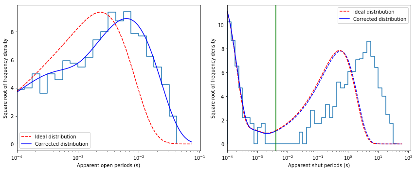
Note that in this record only shut time intervals shorter than critical time (\(t_{crit}\)) were used to minimise likelihood. Thus, only a part of shut time histrogram (to the left from green line, indicating \(t_{crit}\) value, in the above plot) is predicted well by rate constant estimates.